Archive for the ‘VStar’ Category

Polynomial fit to estimate a Mira maximum

July 18, 2012

Grant Foster’s book “Analyzing Light Curves: A Practical Guide” (section 5.5) gives an example of using polynomials to determine critical points of a light curve, in particular: a Mira maximum.

The book addresses the question of how to determine minima/maxima, especially in the presence of scatter in the data. The following figure shows a 7 degree polynomial fit for a Visual JD range around maximum for Mira.

Polynomial fit of degree 7 for a Mira minimum

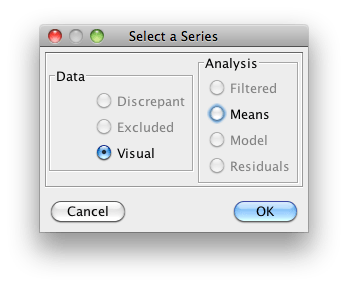
To obtain this plot, load the data from the AAVSO International Database for the JD range shown (2451460.0764 to 2451559.539), select Polynomial Fit from the Analysis menu or toolbar, select the Visual series, then the number of degrees for the polynomial, in his case: 7.

VStar series selection

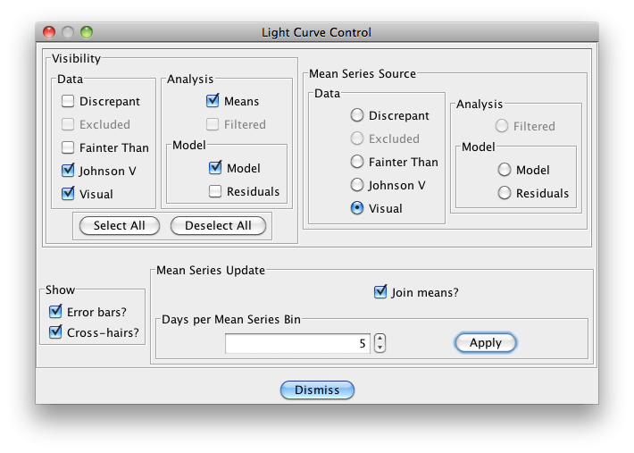
Experiment with the degree value to see the effect upon the least squares polynomial fit. A 5 days-per-bin mean series (again, based upon the Visual series) makes a useful comparison. This can be changed via the View menu’s Plot Control dialog.

Switching to the Model and Means tabs in turn and clicking the Magnitude column to re-order it, allows the maximum value in the series to be easily found. Selecting such a row causes the cross hair in the plot to move also.

Grant’s discussion goes beyond simple polynomial fits, including a discussion of information criteria or “goodness measures” and a consideration of alternatives such as the Lowess smooth, both of which are on the roadmap for VStar. He also spoke about this in more detail at one of the Astro April Citizen Sky talks about uncertainty in determining time of minimum/maximum.

Given that it is currently near maximum, while writing this entry I also created polynomial fits for filtered ranges of R Car, another long period variable. I’ll leave that for another post though.

On a related note, I’ve been asked by a few people recently about when VStar will include a Time of Minimum/Maximum (ToM) capability such as Kwee-van Woerden for use with eclipsing binary light curves. This is working its way higher up the list.

WWZ contour plots

September 15, 2011

In my last post about WWZ I said this:

What VStar does not currently do is create a 2D plot that represents the WWZ statistic as different colours. It’s an open question as to whether this is necessary, but such plots do have a striking appearance and some may prefer them over 3D plots.

I’ve implemented contour plots for WWZ in VStar now. Here is the plot for the T UMi example in that last post.

T UMi WWZ contour plot

T UMi WWZ contour plot

I may tweak the appearance of these plots yet, but this is essentially what they will look like in the forthcoming release.

This is similar to the example plot in Grant’s book on page 235 (Fig 11.14) except that period is on the Y axis rather than frequency. It’s interesting to compare this against where the peaks occur the 3D plot.

I have also added the ability to:

  1. Request WWZ and DC DFT in terms of period range rather than frequency range;
  2. specify the number of time divisions across the dataset range for WWZ. The improvement in time resolution is most noticeable in the contour plot. In the plot above, I used a value of 80 instead of the default of 50.

An internal VStar team testing release is getting close, hopefully by the end of this week.

Weighted Wavelet Z-Transform (WWZ) in VStar

August 30, 2011

It’s hard to believe 6 months have elapsed since the last release of VStar. Although there  is no firm date for the next release yet, there has been a lot of progress towards it. I hope it will happen this month, at first internally to the Citizen Sky VStar team.

My last two posts covered a couple of forthcoming features: model creation from period analysis and the CLEANest algorithm. I used examples from Grant Foster’s book Analyzing Light Curves: A Practical Guide to illustrate the new features. I’m still collaborating with Grant and Doug Welch on improvements to CLEANest such as taking into account the harmonics of specified frequencies. Grant has already incorporated into his R version of CLEANest. This aspect of VStar development has been on the back-burner for the last few weeks so in the meantime I decided to implement Weighted Wavelet Z-Transform (WWZ), also covered in Grant’s book (and created by him). I know that Aaron Price has been looking forward to seeing WWZ in VStar.

Again, I have (with permission from AAVSO) had the benefit of a reference implementation in the form of Fortran code available in the AAVSO Software Directory, just as I did with Date Compensated Discrete Fourier Transform (DCDFT) in the form of the Fortran code of TS (also available via the same software directory web page).

Whereas period analysis algorithms like DCDFT, Phase Dispersion Minimisation, Analysis of Variance (AoV) and others (DCDFT is implemented in VStar) provide information about candidate periods in a time series dataset, and CLEANest refines candidate periods, WWZ analyses how a star’s period changes over time: time-frequency analysis. Grant uses the stars T Umi and R Dor as examples.

The T Umi dataset, taken from the AAVSO International Database (AID) in Grant’s example spans the JD range 2,420,000 to 2,455,000.

Creating a phase plot with periods resulting from DCDFT in VStar doesn’t result in an obviously “clean” fit over the time range. WWZ helps to explain why. Applying WWZ to the dataset requires selecting the series to be analysed, then the following parameters:

  • Minimum frequency
  • Maximum frequency
  • Frequency step or resolution
  • Decay: the wavelet window; smaller values yield better resolution of variation

This post won’t go into detail about these parameters or the WWZ algorithm. Apart from Grant’s book, the HTML docs accompanying the WWZ Fortran code available in the AAVSO Software Directory are worth reading.

For T Umi, choosing values for the above parameters (entered into a dialog box) of : 0.00001, 0.02, 0.00001, 0.001 give the following plot of period vs time:

This is VStar’s equivalent of Figure 11.16 in Grant’s book.

The WWZ result dialog also gives other plots and data tables derived from the result of analysing each frequency in the specified range and interval over a range of times. One of the tables shows only those time-frequency pairs for which the WWZ statistic is at maximum (distance from 1 denotes degree of variation for a particular time) for each time under test.

The following 3D plot shows period and time on two axes as above, but adds the WWZ statistic on the 3rd dimension:

The ridge of the plot denotes the degree of variation at a particular time-frequency (or time-period in our case) pair. In the VStar dialog tab in which this appears, the mouse can be used to rotate this plot and view it from various angles.

What VStar does not currently do is create a 2D plot that represents the WWZ statistic as different colours. It’s an open question as to whether this is necessary, but such plots do have a striking appearance and some may prefer them over 3D plots. WinWWZ, developed by Geir Klingenberg and Lisa Henkel creates such “contour plots”. Grant also talks about the pros and cons of each kind of plot in his book.

What is currently committed in SourceForge is not the last word before the looming release, and I would appreciate feedback on the current interface. I may yet use a different 3D plot library. VStar currently uses JMathPlot for 3D plots and JFreeChart for all other (2D) plots here and elsewhere in the tool.

Grant’s second example is of R Dor in the JD range 2,426,000 to 2,556,000.

With the visual series selected for analysis and the parameters 0.001, 0.009, 0.0001, 0.005, the period vs time plot appears strange:

until you look at the 3D plot (equivalent to Figure 11.16 in the book):

which, as Grant says, shows that R Dor (at least in the JD range under test) exhibits mode switching, i.e. it switches from one pulsation mode to another (between periods of around 332 and 175 days).

I hope you enjoyed this brief look at another of the new features that will appear in the next release of VStar.

BZ UMa model and CLEANest

July 13, 2011

Over the last few days I finished coding and unit testing the multi-period analysis CLEANest algorithm implementation in VStar (again, translated from TS). The main missing parts were allowing the user to specify “variable” and “locked” periods in addition to selecting them from a DC DFT period analysis result. I’m at the point where I need feedback.

Apart from the unit tests that show equivalence with the TS program, I’ve been “playing” with a few different datasets and pre-whitening, modelling, CLEANest.

In my last post, I created  a model based upon two periods found through successive refinement (pre-whitening). Tonight I used CLEANest to obtain those periods for a model with fewer steps.

Starting from the DC DFT frequency scan (low frequency: 0, high frequency: 50, resolution: 0.01) of the BZ UMa V band data, we end up (as last time) with a top hits table like this:

Selecting two periods for CLEANest from BZ UMa DC DFT top hits

Selecting two periods for CLEANest from BZ UMa DC DFT top hits

Also shown is that I have selected the two values used in the two-period model last time before clicking the CLEANest button giving us:

Two periods with same power added by CLEANest to BZ UMa DC DFT top hits

Two periods with same power added by CLEANest to BZ UMa DC DFT top hits

The CLEANest algorithm inserts two new rows at the top with the same highest power. I have selected these above. Switching to the “Power vs Frequency” (power spectrum) tab we see:

Two periods from CLEANest superimposed as "spikes" on BZ UMa DC DFT periodogram

Two periods from CLEANest superimposed as "spikes" on BZ UMa DC DFT periodogram

Notice the spikes showing the refined frequencies from the CLEANest algorithm. Switching back to the Top Hits tabbed pane, clicking “Create Model”, we get:

Two period BZ UMa model from CLEANest

Two period BZ UMa model from CLEANest

I am still quite new to period analysis, including CLEANest (it’s one thing to code it, another to apply it…), so I’m interested in feedback from others regarding the appropriateness of CLEANest in a context like this, and also first impressions regarding usability.

Modelling with VStar

July 10, 2011

Ever since reading Grant Foster’s description of modelling in Analyzing Light Curves: A Practical Approach, I’ve been keen to incorporate this functionality into VStar. In recent SourceForge commits I’ve implemented a first cut of this.

If you are happy to “live on the bleeding edge”, you are welcome to try it now by checking out from the SourceForge Subversion repository or downloading a tarball. Otherwise, it will be available in the next VStar release.

I want to give an example from chapter 10 in Grant’s book: A day in the life of BZ UMa. BZ UMa is a cataclysmic variable that has undergone numerous outbursts; see this Slacker Astronomy video page re: a BZ UMa poster by Aaron Price.

Grant works through an analysis of just one day of BZ UMa data that shows short-term periodic changes. In talking with Grant, it turns out that the JD range used for the example is 2,454,205.3 to 2,454,205.9 not 2,445,205.3 to 2,445,205.9 as shown in the book.

Obtaining data in the range 2,454,205.3 to 2,454,205.9 from the AAVSO International Database with VStar, and looking at just the V band data gives this light curve:

BZ UMa V band for the JD range 2,454,205.3 to 2,454,205.9

BZ UMa V band for the JD range 2,454,205.3 to 2,454,205.9

Applying a Date Compensated Discrete Fourier Transform (DC DFT) gives this periodogram:

BZ UMa V band DC DFT

BZ UMa V band DC DFT

Switching to the Top Hits tab shows that the tallest peak corresponds to a frequency of around 14.18 cycles per day (depending upon exactly what frequency scan parameters you provide; I changed the High Frequency to 100 and the Resolution to 0.01 in the period analysis parameters dialog). In chapter 10, Grant suggests creating a model based upon this main frequency. In VStar, clicking the “Create Model” button in the Top Hits pane will create this and plot it against the V band data as follows:

BZ UMa V Model with main frequency of 14.18 cycles per day.

BZ UMa V Model with main frequency of 14.18 cycles per day.

Apart from the model series, VStar also generates a series called “Residuals” which results from subtraction of the model data from the model source series (V band in this case) data that looks like this:

BZ UMa residuals for model of 14.18 cycles per day

BZ UMa residuals for model of 14.18 cycles per day

This so-called pre-whitened data has the main frequency removed from the raw V band data. Section 8.6 of Grant’s book is about pre-whitening.

The question then is whether period analysis of the residuals would reveal further signal. A DC DFT of the BZ UMa residuals above gives this periodogram:

BZ UMa DC DFT of residuals from 14.18 cycles per day model

BZ UMa DC DFT of residuals from 14.18 cycles per day model

This power spectrum shows a Top Hit of around 28.36. In the light of this additional frequency, Grant suggests creating a model based upon two frequencies, in this case: 14.18 and 28.36. You can of course create a model based upon just this new frequency:

BZ UMa Residuals Model

BZ UMa Residuals Model

Now, one of the current limitations of VStar’s implementation of modelling is that you cannot incrementally add to an existing model or combine two or more. I definitely intend to permit both however, in addition (a little later) to the construction of arbitrary models. For now, the best we can do in VStar is to return to the initial V band DC DFT and select two frequencies that are close to these (in this case: 14.18 and about 28.58) giving this model plotted against the V band data:

BZ UMa V band two-frequency model

BZ UMa V band two-frequency model

VStar’s Analysis menu now has a Models item that opens a dialog when selected containing a list of created models. They can be selected for re-plotting or deletion. Only one model-residuals series pair can be viewed at a time. Note also that new tabs in the main VStar window contain tables of the model and residual data. Polynomial fits and their residuals are now also included in the models dialog box.

Of course, model and residual data can also be included in a phase plot. In order for a model to make sense for some stars (e.g. del Cep), a phase plot is pretty much mandatory; not so for the current BZ UMa example.

Grant goes on to use the residuals from this model to identify additional harmonics beyond the fundamental frequency and first harmonic mentioned above to further refine the model. His analysis also adjusts for two groups of observer bias to compensate for consistently different estimates by two observers. VStar’s filter feature can be used to illustrate one such bias group:

BZ UMa Observer aBias

BZ UMa Observer aBias

As mentioned already, VStar’s current modelling capability does not yet permit such refinements as observer bias to be included in the model. In any case, I hope this example has provided some insight into where VStar’s modelling functionality is heading.

2011 AAVSO Director’s Award for little old me

May 27, 2011

I was very happy, and humbled, to be told this week that I’m the recipient of the 2011 AAVSO Director’s Award for leading the development of VStar, an open source variable star data visualisation and analysis tool. It’s humbling when you look at the predecessors of the award.

You can learn more about VStar, and the context in which it got started, at CitizenSky. I have not developed VStar alone. I’ve had help from domain experts, AAVSO staff, and other developers.

If you want to try VStar, just click the green Download button on the SourceForge page. If you have Java 1.6 or higher installed on your Windows, Mac, Linux, or OpenSolaris machine, the latest version of VStar will be downloaded and run (via Java Web Start technology).

VStar is still an active, ongoing project. There’s plenty left to do. One key area of focus right now is the addition of a modelling capability and more period analysis functionality. If you are a developer looking for an interesting Science-related project to contribute to, try it out and have a look at the SourceForge bug & issue tracker to see if anything interests you.

Data analysis (e.g. finding periods in variable star data) is a growth area for amateur astronomers. VStar is growing into a tool that makes that easier to get into.

Now, back to coding… 🙂

Second Citizen Sky Workshop and ASV Talk

September 12, 2010

From September 2nd to 5th I participated in the second Citizen Sky workshop in San Francisco, attended by a mix of professional astronomers, amateur astronomers, and Science educators. The event was held at the California Academy of Sciences (CAS) in Golden Gate Park.

On the way back home I gave a talk about Citizen Sky and VStar to the Astronomical Society of Victoria as part of the yearly ASSA/ASV speaker exchange. I was made to feel welcome by members of the ASV, some of whom took me out to dinner prior to the meeting. I appreciated the opportunity to give this talk, which seems to have been been well received.

The San Francisco workshop was packed with sessions but we had two hour lunch breaks encouraging lots of interaction between participants.

I gave two talks: a practical VStar session and a summary of the VStar Team’s activities. The team gained a few new members during the workshop. See the VStar Team page for more details.

There was plenty of interest and discussion regarding VStar throughout the workshop with a couple of professional astronomers and a new data analysis group (formed during the workshop) planning to make use of the tool for specific projects.

Some Citizen Sky participants adopting the VStar pose after the last session (courtesy Joan Chamberlin, pictured 2nd from left next to the author).

Some Citizen Sky participants adopting the VStar Pose after the last session. Courtesy Joan Chamberlin, pictured to the left of the author.

Use of VStar by a participant with a European locale revealed an important class of bugs that needs to be fixed relating to numeric input when VStar is used on machines configured with non-English locales. It’s something I knew I had to address, but being presented with it by a user has raised its priority in the SourceForge tracker.

The workshop agenda was diverse and, apart from the sessions mentioned above, included topics such as:

  • Update on the status of the Epsilon Aurigae eclipse
  • Disks in astrophysical objects
  • Evolutionary status of the binary based upon recent measurements
  • Analysis of Epsilon Aurigae spectrum monitoring by a college (San Mateo) student team
  • Precision, accuracy, and uncertainty in data
  • Light curves of different types of variable stars
  • Basic and intermediate time series data analysis
  • Choosing topics for Scientific investigation
  • Scientific paper writing

All sessions were captured on video, and will be made available, along with the accompanying slides, on the Citizen Sky website.

One of the CAS roof-top garden domes.

One of the CAS roof-top garden domes.

Participants had the opportunity to see two shows in the CAS Morrison Planetarium, in addition to the premiere of the Citizen Sky planetarium trailer.

Morrison planetarium dome

Morrison Planetarium dome

I also had a bit of time to look around San Francisco and was fortunate to see the Golden Gate Bridge when it was clear of fog. Joan Chamberlin (leader of the Southern Gems Team) and I took a walk on the bridge and had wonderful views of the Bay.

David on the Golden Gate Bridge, September 2010

Author on the Golden Gate Bridge

Attendance at the second Citizen Sky workshop came after months of VStar development in my spare time. It was great to get together again with people I’d met at the first workshop in Chicago last year, as well as getting to know new people.

Dinner out after the last day of the workshop

Dinner out after the last day of the workshop

Other than catching up on sleep, there is still plenty of work remaining to further improve and extend VStar and to apply it to data analysis activities emerging from the second Citizen Sky workshop.

Apart from the palpable general sense of camaraderie, a participant named Bob Miller captured the spirit of those assembled at Citizen Sky via the debut of his song We are the stars, a video of which was played just before lunch on the second day of the workshop.

Bob Miller at Citizen Sky 2

Bob Miller at Citizen Sky 2

Other than catching up on sleep, there is still plenty of work remaining to further improve and extend VStar and to apply it to data analysis activities emerging from the second Citizen Sky workshop.

If you are in the least bit interested, I would suggest monitoring the Recent Posts section of the Citizen Sky site, and of course, feel free to ask me for more information.

I want to say a big thanks to Rebecca Turner, Aaron Price, and AAVSO in general for organising the workshop. It was awesome.

NACAA 2010 VStar workshop summary

April 12, 2010

Here’s the NACAA 2010 VStar workshop summary I recently posted to Citizen Sky:

http://www.citizensky.org/teams/vstar-software-development/vstar-nacaa-2010-workshop-summary

VStar and Eps Aur talks at ASSA and NACAA

March 27, 2010

On February 3 this year I gave a talk about VStar and the “star” of the Citizen Sky project, Epsilon Aurigae, at the monthly general meeting of the Astronomical Society of South Australia (ASSA). Here are the slides as PDF and PowerPoint.

Next Friday (April 2 2010), I’m running a half day VStar workshop and presenting a poster at the National Australian Convention of Amateur Astronomers (NACAA) in Canberra, Australia. I’ll give a summary after the event.

VStar development update

December 31, 2009

VStar development has continued since my August entry after returning from the first Citizen Sky workshop. For the last several weeks, the VStar Development Team has been been making weekly releases that are available via WebStart (TM) from the Citizen Sky VStar Team page (see “Download VStar Now” button).

See also the SourceForge site for more information regarding ongoing activities.

My main focus is still upon code and unit test. Phase plots can be created but further integration with all views is required. This has most of my attention at the moment but numerous other bugs and improvements have also been addressed (see bug and feature tracker).

The plan for the early New Year is to bring phase 1 to an end and move on to period analysis and other functionality.

This and other matters were discussed during the annual AAVSO meeting in Boston in November into which I Skyped for a VStar session. Sara Beck, Michael Umbricht, Grant Foster (developer of the original VStar), and from photometrica.org, Geir Klingenberg and Michael Kran. The possibility of adding photometrica as another data source to VStar was discussed. Grant shared his ideas regarding period analysis algorithms. Michael Umbricht also gave a presentation about VStar to AAVSO meeting attendees.

A  relatively recent development is that along with AAVSO staff members and Michael Umbricht, I’m an author on a poster paper to be presented by Arne Henden at the January meeting of the American Astronomical Society: “Statistical Software Development as an Example of a Citizen Sky Participant Team”.

In February 2010, I will be giving a talk to the Astronomical Society of South Australia about VStar, Citizen Sky, and Epslion Aurigae.

I would again like to acknowledge the ongoing assistance of Sara Beck, Michael Umbricht, Adam Weber, others at AAVSO and Citizen Sky participants who are using VStar.

All the best for the New Year.